Hoverman HDTV UHF antenna
| Antenna Overview |
| VHF (2m/MURS) |
| Moxon Rectangle |
| Yagi-Uda |
| High-Gain Omni |
| UHF (70 cm) |
| Dual-Rectangle |
| HDTV |
| Hoverman |
| Gapless Hoverman |
| Extended Hoverman |
| jed |
| S-Lang |
| most |
| Complex Domain Coloring |
| SLxfig |
| Antennas |
| Thermochron |
| Main Page |
The Hoverman antenna was invented in the 1950s by Doyt Hoverman before the advent of computer modeling, and appears to be a variation for UHF of the much earlier Chireix-Mesny shortwave antenna. In late 2007 and through much of 2008 the Hoverman antenna was subjected to computer modeling and a number of improvements were made by a small group of antenna enthusiasts on the digitalhome.ca forums. The resulting design was dubbed the ``Gray-Hoverman'' antenna. You can read more about the history of this design on their web page.
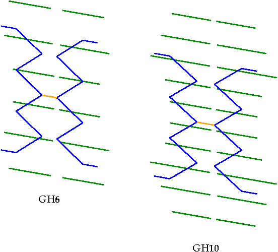
| The models presented below are my second revision (``rev-2'') to first (GH6) and second generation (GH10) digitalhome Hoverman designs (represented as ``rev-0'' in the plots). The GH6 utilizes 6 pairs of half-wave reflectors, while the GH10 has 10 pairs of half-wave reflectors. Schematics of the rev-1 versions of these antennas are shown below. Also included are designs for 4 and 8 pair models, as well as a narrow and wide-band version of this antenna. |
ContentsPerformance PredictionsSpecifications NEC-2 Files Monte-Carlo Simulations A Narrow-Band Hoverman A Wide-Band Hoverman |
Performance Predictions
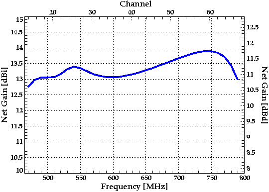
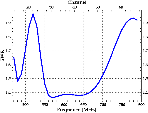
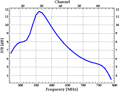
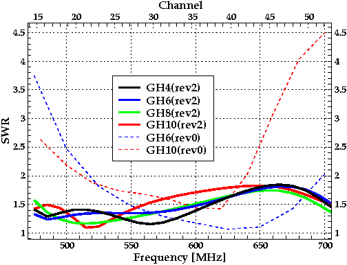
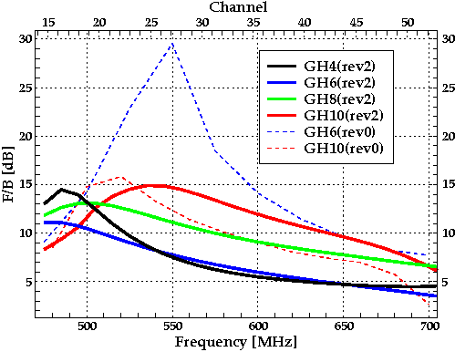
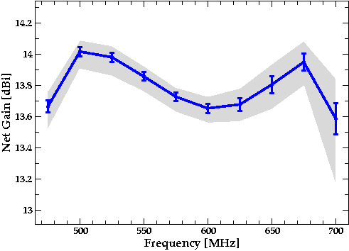
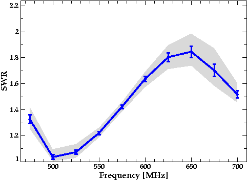
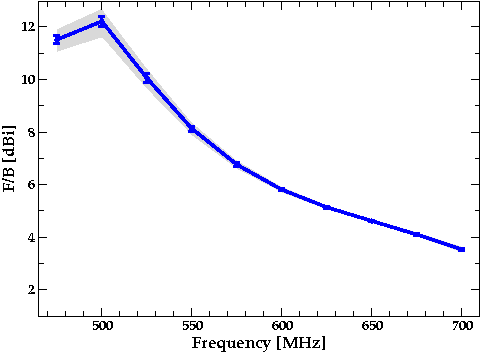
The following plots show the net gain (corrected for the SWR effects), front-to-back ratio, and the SWR across the post-February 2009 UHF band for the antenna geometries described below. In all these plots, the (rev-2) designs presented here are represented by the solid curves, while the dashed curves denote those of the original (rev-0) models described on the Gray-Hoverman web page and its forums. The rev-2 designs are a modest (about 1 dB) improvement to my earlier rev-1 versions.
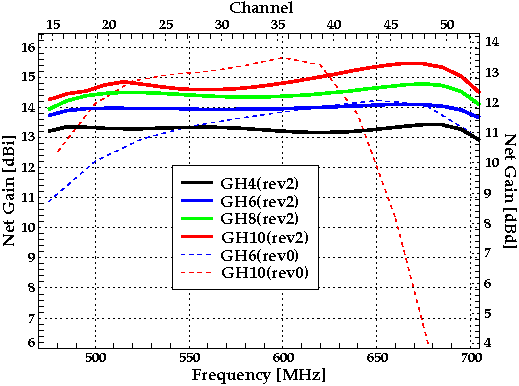
The above plot shows that original digital-home GH10 design performs about a dB better than the GH10 design presented here across the middle of the UHF band, but performs significantly worse on the upper end of the band. The reason for poor performance away from the middle of the band can be seen in the following plot of the SWR plot.
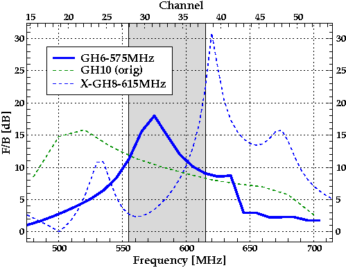
As the following plot shows, the original GH6 model has a very good F/B ratio in the middle of the band, and is much better than the second generation GH10 across the entire band.
Specifications
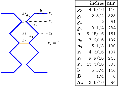
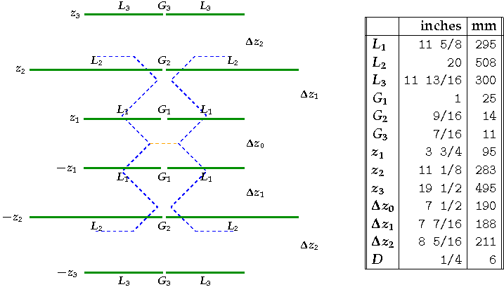
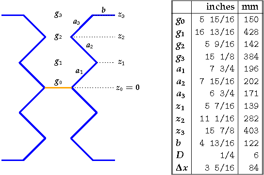
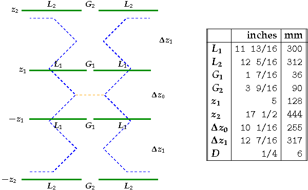
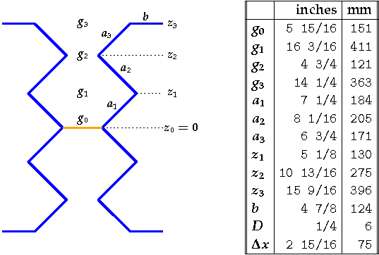
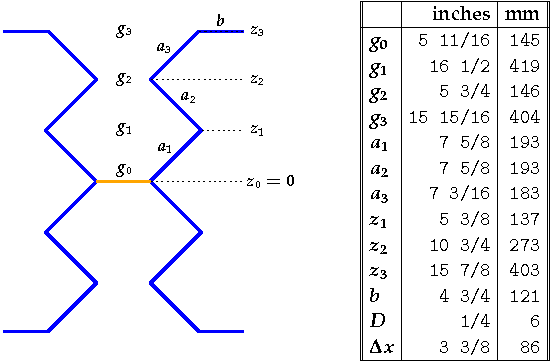
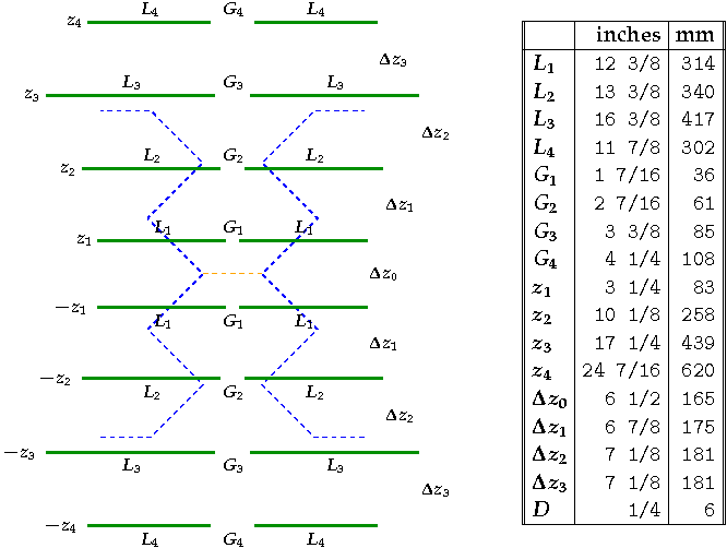
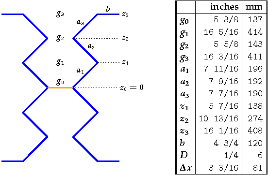
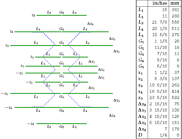
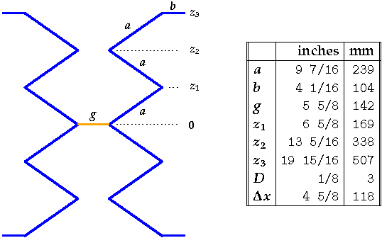
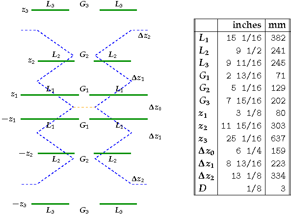
The geometric parameters of the GH6 and GH10 were found by the optimization process outlined on the Antenna Overview page. Each antenna consists of two parts: a driven element formed by a zigzag pair, and a reflector made up of a varying number of horizontal parasitic elements.
The figures and tables provided below give the detailed geometric information about the antennas. The measurements have been rounded to the nearest 16th of an inch, as well as to the nearest mm. Each of the tables contains a ``D'' parameter, which represents the diameter of the wire to be used. In addition, the tables for the zigzag driven element contains a `` Δx'' entry that represents the spacing between the driven element and the reflector. The `` Δz'' values that appear in the reflector geometry tables represent distances between adjacent reflector rods. For example, z2 = z1 + Δz1. (The symbol Δ is commonly used in mathematics to signify a difference between two values. In this case Δz1 = z2 - z1.) All distance values appearing in the tables refer to the centers of the corresponding elements.
The feedpoint, denoted by the orange segment connecting the zigzag pairs, has a 300 ohm impedance. As such, a 300 ohm matching transformer will be required to connect this to standard 75 ohm cable (RG-6).
GH4 Parameters
GH6 Parameters

GH8 Parameters
GH10 Parameters
NEC-2 Files
In this section, links are provided to the NEC-2 files for the above designs. These files require a version of NEC-2 that is able to read geometry lines that consist of more than 80 bytes. Standard versions of NEC-2 are not able to do this and may produce a geometry card error when used with these files. I use a version of nec2dx that I modified to read geometry cards up to 256 characters in length.
Monte-Carlo Simulations
To what tolerances must one build the antennas to achieve the predicted gains? Stated another way, how robust are the antennas to construction errors? In order to shed some light on this question, I simulated 500 random (rev-1) GH6 antenna geometries where each differed from the recommended geometry by a random amount. In particular, each dimension X was perturbed by a uniform random value between -1/8 and +1/8 of an inch. The resulting distribution of net-gains, SWRs, and F/B ratios are given in the plots below. In each of the plots, the solid blue line represents the mean value observed. The error bar gives the standard deviation from the mean, and the shaded region delineates the minimum and maximum values observed. As the plots show, the antenna appears to be quite tolerant of construction errors on the order of plus or minus 1/8 of an inch (3 mm).
A Narrow-Band Hoverman
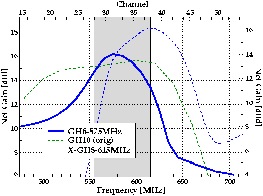
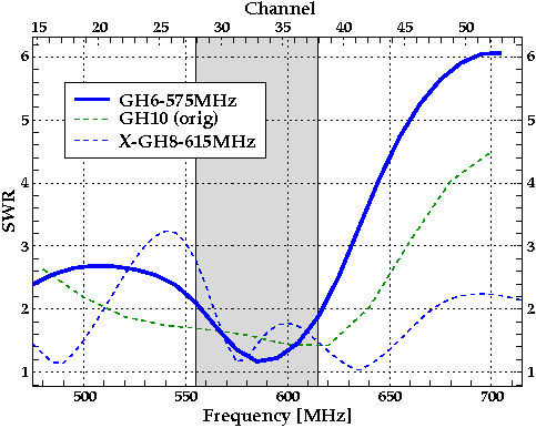
As the above plots of the net gain show, the Hoverman antenna has a very wide bandwidth making it an appealing UHF antenna. On the other hand, it is possible to optimize the Hoverman antenna for a particular frequency. The 6-pair reflector design presented below was optimized for the maximum net gain at 575 MHz, where modeling indicates that it has a respectable net gain of more than 16 dBi. As this design has a much narrower bandwidth, it should only be used for fringe reception of a few channels near its design frequency.
I have had a number of requests for this antenna for use at other frequencies. If you want to adapt this design for use at a frequency other than 575 MHz, then simply scale the geometric measurements in the tables below by 575 MHz divided by the desired frequency. For example, to use the antenna at 525 MHz, multiply all the measurements by 575/525 = 1.095. In this case, a value such as 300mm in the table would become 329mm, or 12 and 15/16 inches. This scaling applies to all the numbers.
The plots below compare the predicted performance of the narrow-band GH6 to that of the second generation GH10 from the digital home site. Also shown for comparison is the predicted performance of the Extended Hoverman, which was optimized for 615 MHz. The shaded area corresponds to the frequency range where the SWR of the narrow-band design is less than two.
Here are the geometric values for the narrow band GH6. For values at other frequences, use the scaling rule described above.
A Wide-Band Hoverman
The above geometries were designed for the post-February 2009 UHF band, which has a frequency range of 470-698 MHz. This section contains the design parameters for a 6-pair reflector model that spans the broader frequency range of 470 MHz to 794 MHz.